Light data analysis

To understand the nature of the data better, we first do some light data analysis.

data_dir = 'Physics_2020_Dimensions'
df = pd.read_pickle(os.path.join(data_dir, 'dimensions_data_clean.pkl')) 

print('Altogether we are dealing with a total of {} publication items in the category Physical Sciences published in the year 2020'
      .format(len(df)))


all_labels_full = [item for sublist in df.Labels_str.values.tolist() for item in sublist] 
all_labels = list(set(all_labels_full))

multilabel_combs = (set([' '.join(sublist) for sublist in df.Labels_str.values.tolist()]))

print('\nThese are the {} subfields we are dealing with:\n'.format(len(all_labels)))
print(', '.join(all_labels))
print('\nIn the dataset these 10 labels are distributed over {} different multilabel combinations.'.format(len(multilabel_combs)))

Altogether we are dealing with a total of 140717 publication items in the category Physical Sciences published in the year 2020

These are the 10 subfields we are dealing with:

Nuclear and Plasma Physics, Synchrotrons and Accelerators, Astronomical Sciences, Medical and Biological Physics, Quantum Physics, Space Sciences, Classical Physics, Particle and High Energy Physics, Atomic Molecular and Optical Physics, Condensed Matter Physics

In the dataset these 10 labels are distributed over 96 different multilabel combinations:

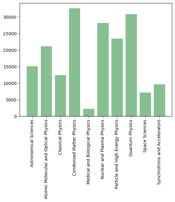
Visualize the distribution of the publication items over the different subfields. The distribution is quite heterogenous with the highest number of publication items labeled Condensed Matter Physics and the lowest number of items labeled Medical and Biological Physics.

labels, counts = np.unique(all_labels_full, return_counts=True)

fig, ax = plt.subplots()

ax.bar(labels, counts, align='center',color='#86bf91')
ax.set_xticks(ax.get_xticks())  # just get and reset whatever you already have to avoid a bug in matplotlib
ax.set_xticklabels(labels, rotation=90)

plt.show()

Remember that we are dealing with a multilabel classification. To get a feel for the distribution of the number of different labels per item in the dataset we plot the distribution.

labels_nr = df.Labels_num.apply(lambda x: len(x))
df = df.assign(Labels_nr=labels_nr.values)

df.hist(column='Labels_nr', bins=4, grid=False, color='#86bf91', rwidth=0.9, figsize=(3,4))
plt.show()

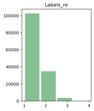
In the majority of cases the publications are assigned to only one subfield, about a quarter of the items has two labels, less then 5 percent have three labels, the number of items with four labels is insignificant, no publication item is assigned to more than 4 subfields.

Quickly inspect the co-occurence graph of the labels:

G = nx.from_edgelist((c for n_nodes in df.Labels_str.values.tolist() for c in combinations(n_nodes, r=2)),
                     create_using=nx.MultiGraph)

# visualize graph
fig, ax = plt.subplots(figsize=(20,20))

pos = nx.draw_spring(G, with_labels = True, ax=ax)

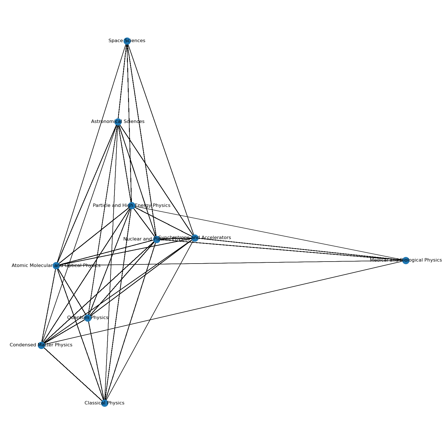
The co-occurence graph is not too informative, as expected Space Sciences and Astronomical Sciences have very similar co-occurrences. Medical and Biological Physics and Classical Physics stand out somewhat as they never occur together, and likewise not with either Space Sciences or Astronomical Sciences.

Further analysis of the co-occurence of labels:

# pearson correlation for label combinations
single_label_corr = single_label_bool.corr(method = "pearson")

# frequency for label combinations
labels_int = single_label_bool.astype(int)
labels_freq_mat = np.dot(labels_int.T, labels_int)
labels_freq = pd.DataFrame(
    labels_freq_mat,
    columns = all_labels,
    index = all_labels
)

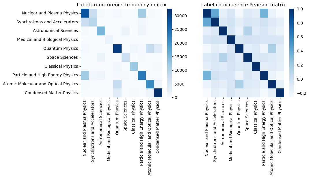
The frequency matrix of label co-occurences:

labels_freq

	Nuclear and Plasma Physics	Synchrotrons and Accelerators	Astronomical Sciences	Medical and Biological Physics	Quantum Physics	Space Sciences	Classical Physics	Particle and High Energy Physics	Atomic Molecular and Optical Physics	Condensed Matter Physics
Nuclear and Plasma Physics	28159	7605	603	73	743	289	307	11872	621	298
Synchrotrons and Accelerators	7605	9626	113	77	78	10	4	1388	161	29
Astronomical Sciences	603	113	15094	0	21	1981	4	1516	151	4
Medical and Biological Physics	73	77	0	2217	0	0	0	2	4	5
Quantum Physics	743	78	21	0	30787	0	1317	863	7981	3882
Space Sciences	289	10	1981	0	0	7170	0	435	5	0
Classical Physics	307	4	4	0	1317	0	12389	208	281	488
Particle and High Energy Physics	11872	1388	1516	2	863	435	208	23423	271	147
Atomic Molecular and Optical Physics	621	161	151	4	7981	5	281	271	21142	1671
Condensed Matter Physics	298	29	4	5	3882	0	488	147	1671	32562

Co-occurence of labels; frequency and Pearson matrices as a heatmaps:

import seaborn as sn
fig, (ax1, ax2) = plt.subplots(1,2,figsize = (10,4))
ax1.title.set_text('Label co-occurence frequency matrix')
ax2.title.set_text('Label co-occurence Pearson matrix')
sn.heatmap(labels_freq, cmap = "Blues", ax=ax1)
sn.heatmap(single_label_corr, cmap = "Blues", ax=ax2, yticklabels=False)
plt.show()